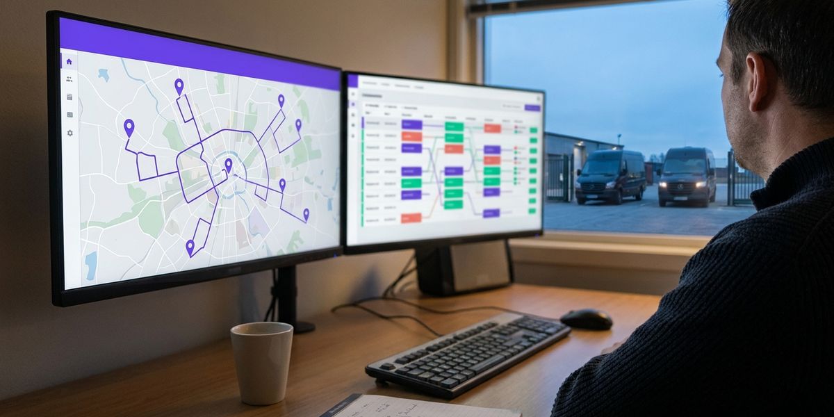
A dispatcher running a 12-route corporate shuttle network on a Tuesday morning has roughly forty minutes to decide whether to add a vehicle, reshuffle three pickup sequences, or accept a dozen late drop-offs. The HRIS rosters changed overnight; one driver called out; a weather alert just shifted demand onto the heavier T/W/Th peak the Census Bureau’s 2024 commute data already flagged at 27.2 minutes mean one-way travel time. The dispatcher knows the network well enough to pick a good answer. They cannot pick the best one. Possible route assignments across twelve vehicles, eighty stops, and four shift windows run into the hundreds of millions, and no human evaluates that space before the 7:15 a.m. departure.
That gap between “a good plan” and “the best feasible plan” is what route optimization software is for. The math is older than most readers expect, the formulations are more varied than vendors usually admit, and the cases where it pays back are bounded in ways finance teams need to understand before signing a contract. This guide is written for ops directors, fleet managers, and mobility program managers at employers in the 200-20,000+ range, and for the engineering leaders deciding whether to build, buy, or partner. Consumer turn-by-turn navigation, hailing apps, and long-haul intermodal freight planning sit outside the scope.
What route optimization actually is, and what it isn’t
Route optimization is the computational problem of assigning a set of vehicles to a set of stops, in a sequence, that minimizes one or more objectives (distance, time, cost, emissions) while honoring a set of hard constraints (vehicle capacity, time windows, driver hours, precedence relationships) and soft preferences (rider stop preference, equity across drivers, balance across depots). It is not route planning, which is the unaided act of writing down which vehicle visits which stops. Route planning produces a plan; route optimization produces the best feasible plan a solver can find inside a stated time budget.
The Federal Transit Administration’s definition of microtransit captures the dynamic-routing case directly: “a technology-enabled service that uses multi-passenger vehicles to provide on-demand services with dynamically generated routing” (FTA Report No. 0269, Sep 2024). That definition matters because it draws the line at “dynamically generated.” A fixed corridor with published times and a roster spreadsheet is not microtransit, and a single-stop courier dispatch is not a VRP. Both might benefit from better route planning. Neither needs a route-optimization solver.
Three other distinctions sharpen procurement conversations. Route optimization is not GPS navigation - turn-by-turn directions handle a single origin-destination pair on the road network, while a VRP solver assigns many origin-destination pairs across many vehicles. Route optimization is not fleet management - the telematics layer that tracks fuel, brake wear, and engine-fault codes is an input to a router, not its product. And route optimization is not dispatch in the human sense; a good solver produces a plan, but a dispatcher still has to handle the cancellation, the missed pickup, and the driver who needs a bathroom break.
When the problem really is a vehicle-routing problem, the structure is unforgiving. Capacity is finite. Time windows do not flex. Driver shifts have hard ends. Pickups precede deliveries. Every constraint removes options from the search space, and the size of that space - even for a modest twelve-vehicle, eighty-stop network - puts a brute-force enumeration well past what any operator can attempt manually. Route optimization is the discipline of searching that space efficiently enough to produce a workable plan before the vehicle has to leave the depot.
The math underneath: a short tour of the Vehicle Routing Problem family
The Vehicle Routing Problem first appeared in print under a different name. George Dantzig and John Ramser, writing in Management Science Vol. 6 No. 1 in 1959, published “The Truck Dispatching Problem” - a linear-programming formulation for routing petrol trucks from a central terminal to a set of service stations. The paper has been cited more than 3,700 times across the operations-research literature since. Five years later, Clarke and Wright published the savings algorithm in Operations Research, a constructive heuristic that remains, sixty years later, a baseline implementation inside many commercial routing packages. The field has built outward from those two papers ever since.
Modern operators do not need to write a solver from scratch. They do need to recognize which formulation matches their actual problem, because the wrong formulation guarantees a mediocre result no matter how good the solver behind it. The canonical reference work is Toth and Vigo’s Vehicle Routing: Problems, Methods, and Applications (SIAM, second edition 2014), which catalogues the family in detail. The six variants below cover most operator situations.
| Formulation | What it models | Typical operator case |
|---|---|---|
| TSP (Travelling Salesman) | One vehicle, many stops, return to depot | Single-driver service route |
| CVRP (Capacitated VRP) | Many vehicles with capacity limit, many stops | Beverage distribution, parts delivery |
| VRPTW (CVRP with Time Windows) | CVRP plus hard pickup/drop time windows | Corporate shuttle, school bus |
| MDVRP (Multi-Depot VRP) | Vehicles assigned across multiple depots | Multi-site employer, regional logistics |
| OVRP (Open VRP) | Vehicles do not return to depot | Owner-operator courier, end-of-day rentals |
| PDP / DARP (Pickup-Delivery / Dial-a-Ride) | Paired pickup and delivery, with rider time windows | On-demand shuttles, NEMT, patient transport |
The mismatches are the expensive part. A corporate shuttle operator running fixed daily roster routes does not have an Open VRP - shuttles return to depot. A NEMT provider routing wheelchair-accessible vehicles between patient homes and clinics is solving DARP, not CVRPTW, because rider waiting time and direct-trip ratios matter as constraints in their own right (Cordeau & Laporte, 2007; arXiv survey, 2024). A logistics fleet sending vans from three suburban depots to a shared customer base is MDVRP. Buying a solver labelled “VRP” without checking which subset it implements is how procurements end up with overrides at 30% of dispatched routes within ninety days.
Two more formulations are worth knowing by name. Stochastic VRP models uncertainty in travel time or demand - what most real shuttle operations face during a Wednesday morning rain event. Dynamic VRP re-optimizes during the day as new bookings, cancellations, or traffic data arrive - the formulation behind almost every credible “on-demand” platform. The Solomon benchmark set (56 VRPTW instances of 100 customers each, hosted by SINTEF) lets buyers ask a vendor: how do you score against Solomon C1, R2, RC? The vendors with real solvers will quote scores.
Fixed routes, dynamic routes, and the spectrum between them
Most route-optimization debate in 2026 collapses into a fixed-vs-dynamic argument that gets the question wrong. The right question is which combination suits a particular network’s demand pattern, and the answer is rarely either extreme.
Fixed routes run a published timetable along a published corridor. They scale beautifully when demand is predictable and dense: a manufacturing shift change, a hospital night-shift loop, a hub-and-spoke commuter pattern. Microsoft’s Connector remains substantially fixed because Redmond demand is predictable. The service launched in September 2007 with 5 routes and 12 buses (Microsoft Source, 2007), and by 2016 had grown to 19 routes and 53 buses moving roughly 2,160 round-trip riders a day (Seattle Times, 2017). Boston Public Schools’ BiRD algorithm, developed by Bertsimas, Delarue, and Martin at MIT, optimizes fixed school-bus routes and produced $5M in annual savings with a 50-bus fleet reduction by improving the route plan, not by going dynamic (INFORMS Interfaces, 2020).
Dynamic routes route vehicles against live demand. They win when demand is dispersed, time-window-sensitive, or volatile - a hybrid-work tech campus where Wednesday peaks at twice the Friday volume, a first-and-last-mile shuttle feeding a fixed-route bus station, a non-emergency patient-transport service whose riders book that morning. NJ TRANSIT’s MicroLink, launched April 6, 2026 in Monmouth and Bergen counties under a $7M FTA grant, is a textbook dynamic case: 6 a.m. to 8 p.m. weekday service, first-and-last-mile pickup to fixed-route stops, dispatch handled by an integrated routing engine (NJ TRANSIT).
Between those extremes sits the hybrid network - fixed trunk lines on the densest corridors, dynamic vehicles on the long tail. Hybrid is the right answer for most large multi-site employers. Ryde’s smart shuttles capability covers fixed and hybrid configurations with optimization running across both layers under a single rider data model.
Three operating-model rules survive most arguments. Below 8-15 riders per origin cluster, dynamic almost always loses to a sensibly placed fixed stop. Above 40 riders per corridor per shift, fixed almost always wins on cost per rider-trip. The interesting zone is between, where the hybrid mix - and how the routing engine handles vehicle rebalancing between fixed and dynamic legs - is what separates good platforms from underperforming ones. Microsoft and Seattle Children’s pushed the public-integration version further with a shared-stop pilot using King County Metro infrastructure (Seattle Times) - the line between private routing and public-transit routing is more porous than vendor marketing usually frames.
Where route optimization is being applied today
Five named programs do most of the credible publishing on route-optimization outcomes. They cover delivery, school transport, employee commute, on-demand transit, and patient transport, and they are the cases buyers should know by name when evaluating vendors.
UPS ORION (On-Road Integrated Optimization and Navigation) is the marquee logistics deployment. UPS disclosed that since ORION’s full rollout, the system has saved roughly 100 million miles and 10 million gallons of fuel a year, with about 100,000 metric tons of CO2 avoided annually (UPS, January 2020). ORION evaluates more than 200,000 routing options per driver per day. INFORMS awarded UPS the 2016 Franz Edelman Award for the ten-year research-and-deployment effort that produced it. The 2020 launch of Dynamic ORION added in-day re-optimization; UPS later disclosed that the dynamic extension shaves another 2 to 4 miles per driver per day on top of the original system.
DHL Greenplan, launched in June 2020 by a DHL-financed start-up built with the University of Bonn’s Research Institute for Discrete Mathematics, claims 70% less computing time than standard tools and up to 20% cost savings compared with standard route-optimization solutions (DHL Group press release, 2020). Those are vendor-published figures; the underlying academic credentials of the Bonn discrete-math institute give them more weight than typical marketing claims, but a buyer should still ask Greenplan how the numbers were measured and against which baseline.
Boston Public Schools and the MIT-developed BiRD algorithm is the cleanest publicly documented academic-to-deployment case in school transport. Bertsimas, Delarue, and Martin reported a $5M annual saving and a 50-bus fleet reduction with maintained service quality in INFORMS Interfaces (2020); a companion PNAS paper (Bertsimas et al., 2019) examines the joint optimization of bell times and bus routing in the same BPS deployment. School bus routing sits at the unforgiving end of VRPTW: hard time windows tied to school bell schedules, capacity tied to seating, and a political constraint on stop locations that most vendor demos quietly skip.
Google’s Bay Area shuttle network is the canonical tech-campus example. Public reporting puts the network at roughly 25 routes covering San Francisco, the East Bay, South Bay, Marin, and the Peninsula, with about 3,500 daily riders and 7,000 daily one-way trips, and 300 daily departures between 6 and 9 a.m. (Critical Sustainabilities, UC Santa Cruz; 7x7 Bay Area). Treat those numbers as approximate scale-of-program; Google has not officially refreshed them in recent disclosures.
Healthcare patient transport uses DARP because the constraint set differs from commuter routing - paired pickup and drop-off, narrow waiting tolerances, direct-trip-ratio requirements that prevent operators from sweeping a sick rider through several other stops. A PMC-published hospital case study reported meaningful reductions in non-emergency patient-transport cost and improvements in on-time performance after a VRP-based scheduling rollout, with real-time tracking and data-driven dispatch as the operational backbone (PMC, 2024). One case, not an industry benchmark, but the upside is real when a chronically over-running schedule meets a proper formulation.
A closing note for fleet operators. Empty miles run 15-20% across US trucking; ATRI’s 2021 update put deadhead at 20.6% of miles among all carriers in 2020 and 26% among private fleets. Cutting that line is the most legible win a routing program can deliver. NJ TRANSIT MicroLink and Microsoft Connector both show the pattern most large employers will end up running: private routing layered on top of public infrastructure, not replacing it.
The six categories of constraint that determine the result
Solver quality matters less than constraint definition. A merely good solver fed a precise constraint specification beats a great solver fed a sloppy one nine times out of ten. Six categories cover most real shuttle and fleet networks, and operators evaluating vendors should be able to describe each one for their own program before the first demo.
Capacity is the easiest constraint to state and the easiest to get wrong. Seat count is necessary but not sufficient; practical capacity is whatever the operator is willing to load given driver-comfort, accessibility (wheelchair tie-down occupies multiple seat-equivalents), and rider-experience thresholds. A 22-seat shuttle running at “100% capacity” with riders standing in the aisle is operating at different effective capacity than one with a hard 22-rider cap.
Time windows separate VRPTW from CVRP. A shuttle picking up a manufacturing shift cannot show up 12 minutes late; the line stops. A patient-transport pickup cannot be 25 minutes early; the rider has not finished dialysis. Pickup, drop-off, and slack tolerances need to be stated in minutes. Vendors who let dispatchers set windows after the route runs are not solving VRPTW. They are letting the solver guess.
Sequencing and precedence matter when one stop must precede another - the pickup-before-delivery rule in PDP, plus operator rules like “the wheelchair rider boards first to avoid double-rotation.”
Driver-hours rules get misspecified most often during procurement. Federal hours-of-service rules, union contracts, and meal-break requirements all carve usable time out of a shift in jurisdiction-specific ways. A solver that ignores them produces illegal plans the operations team rewrites by hand.
Fleet heterogeneity is the multi-vehicle-class constraint - a network with 22-seat shuttles, 14-seat vans, and a wheelchair-accessible vehicle is not the same problem as a single-vehicle-type fleet. The solver has to know which riders can ride which vehicles and which vehicles can serve which stops.
Rider preferences and equity are the soft-constraint category, the one skipped most often during procurement. A rider who repeatedly gets the longest detour stops showing up; equity across riders is a soft objective with hard retention consequences. Same for driver workload balance.
A worked example: a 1,200-employee aviation ground-handling site, three shifts, 22-seat shuttles, eight pickup corridors. Capacity = 22 effective seats per vehicle. Time windows = pickup ±5 minutes, drop-off at gate 15 minutes before shift start. Sequencing = one wheelchair user boards first on the inbound vehicle. Driver hours = 10-hour shift, two breaks. Fleet heterogeneity = mix of 22-seat and 12-seat vehicles for lighter overnight demand. Rider preferences = maximum 8-minute detour on any rider’s direct path. Specify those numbers cleanly and a competent solver produces a workable plan in under a minute. Specify them loosely - “pickup sometime between 6:50 and 7:10” - and dispatchers overwrite 30% of the output within two weeks.
How solvers actually work, without the math
Vehicle routing is NP-hard. That phrase means the time to find a provably optimal solution grows faster than polynomially with the problem size, so for any real fleet the operator has a choice between exact methods that may not finish in time, and heuristic methods that finish quickly with no guarantee of optimality. Toth and Vigo’s SIAM volume catalogues the methods in three broad families.
Exact methods (branch-and-bound, branch-and-cut, branch-and-price) produce provably optimal solutions but stop scaling past a few hundred stops on real-world constraint sets. They suit small static networks where optimality is defensible and runtime is not the binding constraint.
Heuristics (Clarke-Wright savings, nearest-neighbor, insertion methods) produce a workable solution quickly with no optimality guarantee. The Clarke-Wright algorithm from 1964 still ships inside commercial packages because it is fast, gives reasonable answers for CVRP problems, and serves as a baseline a more sophisticated method has to beat.
Metaheuristics (tabu search, simulated annealing, genetic algorithms, large neighborhood search) sit between the two - high-quality solutions on large problems in a manageable time budget by searching the solution space intelligently. Different metaheuristics suit different problem shapes; tabu search can find better solutions with less compute than genetic algorithms for many scheduling problems, while genetic algorithms produce several near-optimal solutions at once when the operator wants alternatives (Cordeau and Laporte, 2004-2005). Most modern commercial solvers blend metaheuristics with exact subroutines and learned components like reinforcement learning for the demand-prediction layer.
Two practical implications for buyers. Strong vendors will quote benchmark scores; weak ones say “we benchmark internally.” And runtime is a real constraint in dynamic routing - a solver that needs 90 seconds to re-optimize after a cancellation will produce stale plans when bookings change every 20 seconds. Ask for re-optimization latency at peak load. The answer separates real dynamic platforms from batch-and-republish systems wearing dynamic branding.
When route optimization won’t help you
A guide that only describes upside is sales collateral. Five situations exist where route-optimization software adds cost without proportionate benefit, and operators in those situations need to know.
Small static fleets (one to three vehicles, fewer than fifty stops per day, a customer base that turns over slowly) almost never recover SaaS spend through routing improvements alone. A competent dispatcher with paper and a spreadsheet hits 90%+ of the optimum on a problem that small. The math on a $20K-$40K annual platform contract does not pencil against the marginal mileage saving. Spend the budget on telematics or a better dispatch headset.
Bad stop data breaks every solver. If half the rider addresses in the system are wrong, the optimizer will route to the wrong places very efficiently. Geocoding, address validation, and rider-confirmed pickup points are prerequisites; layering optimization software on top of dirty data produces worse outcomes than the prior manual plan because the dispatcher’s local knowledge is no longer in the loop.
Demand the fleet physically cannot serve is the most painful failure. If 800 riders want pickup between 6:55 and 7:10 a.m. and the fleet has 6 vehicles of 22 seats, the constraint is capacity, not routing. The solver reports infeasible, the operator adds slack, riders run late, and rider NPS collapses. Public microtransit pilots have logged cost-per-rider well above traditional fixed-route service (Governing); RTD Denver subsidizes only the first $20 of each Access-on-Demand trip, with the rider absorbing any excess (RTD-Denver). Those numbers reflect demand the dynamic-fleet design could not absorb at reasonable density - a failure mode no routing engine can fix.
Political, union, or contractual constraints that override the solver are common in school transport, healthcare unions, and multi-site manufacturing with collectively bargained route assignments. A solver reassigning a senior driver away from a long-held route may be overruled regardless of cost outcome. Operators in these environments need either a solver that can hold those assignments as hard constraints, or they need to accept that gains will accrue inside the politically defended subset, not across the whole network.
Over-optimization that erodes rider trust is the subtle one. A rider whose pickup gets reshuffled three times in a week, whose detour gets longer because their stop happens to be near the cluster’s geometric center, stops trusting the program even when the average cost per trip dropped. Operators chasing solver-reported optimality without weighting rider experience as a soft constraint produce plans that look good on paper and lose ridership over six months. Rider-experience-aware optimization is the most consequential constraint set to get right.
Build, buy, or partner: the economics
Operators with a routing problem have three paths: build internally, buy a commercial platform, or partner with a workforce-transport provider that handles routing inside a broader operating contract. The decision is rarely uniform across an organization; engineering-heavy companies sometimes build first and then buy the second generation when maintenance lands on the on-call rotation.
| Path | Up-front cost | Time to pilot | When it wins |
|---|---|---|---|
| Buy commercial routing software | $20K-$200K/year SaaS | 4-12 weeks | Stable demand, mid-size fleet, no specialized constraints |
| Build custom | $60K-$400K initial; 24-32 weeks | Half a year minimum | Unique constraints, dispatcher override >20%, SaaS spend >$80K |
| Partner with platform + operator | Operating-contract based | 60-90 days for first corridor | Want routing inside a broader workforce-transport program |
Build economics deserve a closer look. Custom route-optimization software runs $60K to $400K depending on formulation depth, integration burden (HRIS, telematics, identity), and how much of the operations workflow gets built around it - 24 to 32 weeks from scoping to pilot (Optym, Ideas2IT vendor analyses, 2024-2025). The buy-vs-build inflection point arrives when dispatcher override rate climbs above 20% of daily routes (the platform is no longer the source of truth) and annual SaaS spend has crossed $80K (build economics start to look defensible). Below those thresholds, the answer is keep buying. Above them, scope a build.
Real solvers need real expertise. Toth and Vigo’s volume runs 463 pages of formulations and methods; a competent in-house implementation requires either a doctoral-level operations researcher or two senior engineers spending six months learning the field. Vendor blogs that pitch routing-as-a-weekend-API understate this in proportion to how much they want the contract.
Partner-based deployments collapse the build question for most non-engineering employers. A workforce-transport platform provides routing as a capability inside the broader operating model, alongside dispatcher tooling, rider app, HRIS integration, and reporting. The route-optimization layer sits inside that stack - not a standalone product but the engine running underneath the smart employee commuting platform. For operators whose problem is “we need a working shuttle program” rather than “we need a routing API to call from our dispatch tool,” partner-based is the cheapest path to a credible outcome.
KPIs that prove the routing program is working
A routing program without KPIs is a vehicle program with a software contract. Six metrics separate “we deployed it” from “it is working,” and operators should set targets before pilot go-live, not in retrospect.
On-time rate (OTR). Trips arriving inside a defined tolerance window divided by total trips. ±5 minutes is a common fixed-route tolerance; ±3 minutes for dynamic pickup ETAs. Target 95% at steady state; expect 85-90% in the first 90 days while routes settle.
Trips per vehicle-hour. A productivity measure that exposes whether the solver is loading vehicles efficiently. Compare against pre-deployment baseline rather than against absolute benchmarks, because vehicle type and corridor geometry vary too much for cross-program comparison.
Cost per completed trip. Operating cost (driver hours, fuel, vehicle amortization, platform license) divided by completed rider trips. Routing improvements show here within two to three months. Programs without movement on this line within 90 days have either a demand problem (capacity mismatch) or a constraint-specification problem (solver running against bad inputs).
Deadhead percentage. Empty miles divided by total miles. ATRI data anchors the range: 20.6% across all US carriers in 2020, 26% in private fleets. Corporate shuttle deadhead runs in a similar range during initial rollout and should fall toward 10-15% as routing matures. Above 20% at steady state, something in the depot-to-first-stop or last-stop-to-depot leg is mis-specified.
Rider satisfaction (NPS or equivalent). Captured through an in-app prompt at month 1, month 3, and month 6 post-rollout. Public-transport NPS benchmarks run low; well-routed corporate shuttle programs should clear +30 within two quarters, with dynamic programs hitting +50 to +70 when dispatch is clean.
Scope 3 Category 7 reduction. The GHG Protocol’s three approved methods (fuel-based, distance-based, average-data) all feed Category 7 employee-commuting emissions - the line item that matters for EU CSRD and California SB 253 reporting (GHG Protocol, Chapter 7). The 2026 EU Omnibus I package raised CSRD thresholds to companies above 1,000 employees and €450M turnover, but the disclosure structure remains. A shuttle program replacing single-occupancy-vehicle trips delivers measurable Category 7 reductions, with the gap conditional on occupancy. Distance-based reporting against a platform-captured rider-mile ledger produces auditable numbers; survey-based estimates do not.
One number to anchor the strategic case: the US Bureau of Labor Statistics reported subsidized commuting was available to 10% of private-industry workers in 2024, rising to 14% in the Northeast and West (BLS, The Economics Daily, April 2025). Demand for employer-sponsored commute programs is growing from a low base. Routing-optimized shuttles are the operational layer underneath any serious employer commute benefit.
What to do next
A routing program that does not pencil at the diagnostic stage will not pencil after the contract is signed. Three actions belong on the operator’s calendar this month.
Pull the rider-and-stop dataset. Home addresses (from HRIS, not self-entered surveys, which drift), shift schedules, existing pickup history. If the data is dirty, fix it before scoping software. Run a candidate corridor analysis - which two or three corridors carry enough density for a fixed trunk line, and what does the dynamic tail look like for the rest.
Agree the KPI targets with finance, operations, and HR before procurement runs. On-time rate, trips per vehicle-hour, cost per completed trip, deadhead percent, rider NPS, and Category 7 reduction need numbers next to them at kickoff. Programs that wait until “we have data” benchmark against the pilot itself. The employee transportation management guide covers a complementary KPI rubric; the cost reduction guide covers the finance-side numbers most CFO models miss.
Pilot one route family, not the whole network. A two-to-four-vehicle pilot on the densest origin corridor surfaces 80% of the integration and constraint-specification work; the dispatcher-override rate over the first six weeks tells the operator whether the solver is fit for the broader rollout. Compare against the customer outcomes published in case studies at comparable site profiles.
The decision in front of ops leaders this year is not whether route optimization is real - the named programs settle that question. It is whether the operator’s own constraint set, data quality, and political environment will let a solver do its work. Diagnose those honestly before signing a contract, and the routing program is positioned to be the cheapest line in the commute budget. Skip the diagnosis, and it becomes another SaaS subscription with limited evidence of impact.
If your team is scoping a workforce-transport program where route optimization sits inside a broader operating model, the smart shuttles capability is the natural starting point - the routing engine, dispatcher tooling, and rider app run as one platform under a single operating contract.
Frequently asked questions
What is the difference between route planning and route optimization?
Route planning is the act of writing down which vehicle visits which stops in which order. Route optimization is the computational problem of finding the best feasible plan inside a stated objective and constraint set. Planning produces a plan; optimization produces the best plan a solver can find within a time budget.
How much can route optimization save on fuel?
Published estimates range from 8% to 25% depending on baseline maturity, fleet type, and constraint mix. UPS ORION’s disclosed 100 million miles and 10 million gallons saved per year translates to a low-double-digit percentage against the prior baseline (UPS, INFORMS, 2016-2020). DHL Greenplan claims up to 20% cost reduction relative to standard route-optimization solutions (DHL, 2020). The lower end is what a typical mid-size fleet should expect; the upper end requires a strong baseline gap and committed multi-year optimization work.
Is route optimization the same as GPS navigation?
No. GPS navigation handles a single origin-destination pair on the road network and produces turn-by-turn directions. Route optimization assigns many origin-destination pairs across many vehicles under capacity, time-window, and other constraints. A GPS app can tell a driver how to get from stop 3 to stop 4; a router decides whether stop 4 should be on this driver’s route at all.
When should I build my own route-optimization software vs buy?
Buy until two thresholds cross: dispatcher override rate above roughly 20% of daily routes (the commercial platform is no longer the source of truth) and annual SaaS spend above $80K (build economics start to compete). Below those thresholds, buying almost always wins. Above them, scope a build with a senior operations-research lead - $60K-$400K up front, 24-32 weeks to pilot, benchmarked against the Solomon instance set before declaring victory (SINTEF). For operators whose underlying problem is “we need a working shuttle program” rather than “we need a routing API,” partnering with a workforce-transport platform collapses the question.
Sources
- FTA Report No. 0269: Providing a Dynamic, Data-Driven Micro-Transit Service — Federal Transit Administration (US DOT), accessed 2026-05-22.
- The Truck Dispatching Problem — Dantzig & Ramser, Management Science (INFORMS), 1959, accessed 2026-05-22.
- Scheduling of Vehicles from a Central Depot to a Number of Delivery Points — Clarke & Wright, Operations Research Vol. 12 No. 4, 1964, accessed 2026-05-22.
- UPS To Enhance ORION With Continuous Delivery Route Optimization — UPS (GlobeNewswire), accessed 2026-05-22.
- Optimizing Delivery Routes: UPS On-Road Integrated Optimization and Navigation — INFORMS, accessed 2026-05-22.
- Greenplan: logistics experts launch powerful algorithm for individual route optimization — DHL Group, accessed 2026-05-22.
- American Community Survey 1-Year Estimates: Commuting — US Census Bureau, accessed 2026-05-22.
- An Analysis of the Operational Costs of Trucking: 2021 Update — American Transportation Research Institute, accessed 2026-05-22.
- Optimizing schools’ start time and bus routes — Bertsimas, Delarue, Jaillet, Martin — PNAS, accessed 2026-05-22.
- From Predictions to Prescriptions in Multistage Optimization Problems — Bertsimas, Delarue, Martin — INFORMS Interfaces, 2020, accessed 2026-05-22.
- Microtransit Has Broad Appeal, Despite Clear Drawbacks — Governing, accessed 2026-05-22.
- NJ TRANSIT to Pilot Microtransit Shuttle Service in Monmouth and Bergen Counties — NJ TRANSIT, accessed 2026-05-22.
- Microsoft Connector: 19 routes, 53 buses later — Seattle Times, accessed 2026-05-22.
- Microsoft Unveils Regional Express Bus Service — Microsoft Source, accessed 2026-05-22.
- Technical Guidance for Calculating Scope 3 Emissions — Chapter 7 — GHG Protocol, accessed 2026-05-22.
- All Aboard! Subsidized Commuting Was Available to 1 in 10 Private Industry Workers in 2024 — US Bureau of Labor Statistics, accessed 2026-05-22.
- Vehicle Routing: Problems, Methods, and Applications (Second Edition) — Toth & Vigo, SIAM, 2014, accessed 2026-05-22.
- Solomon Benchmark for VRPTW — SINTEF, accessed 2026-05-22.
- Enhancing Hospital Efficiency and Patient Care: Real-Time Tracking and Data-Driven Dispatch in Patient Transport — PMC / NCBI, accessed 2026-05-22.
- The Open Vehicle Routing Problem: Algorithms, Large-Scale Test Problems, and Computational Results — ScienceDirect (Computers & Operations Research), accessed 2026-05-22.
- The Dial-a-Ride Problem: Models and Algorithms — Cordeau & Laporte, Annals of Operations Research Vol. 153, 2007, accessed 2026-05-22.
- Patient Transport in Hospitals: A Literature Review of Operations Research Approaches — arXiv literature survey, 2024, accessed 2026-05-22.
- Vehicle Occupancy Factors — Federal Highway Administration, accessed 2026-05-22.
- A first-of-its-kind program: Microsoft, Seattle Children’s shuttles are now using Metro stops — Seattle Times, accessed 2026-05-22.
- Build vs. Buy Optimization: A Decision Framework for Logistics and Routing — Optym (vendor blog), accessed 2026-05-22.
- Build Route Optimization Software: Cost, Stack and Timeline — Ideas2IT (vendor blog), accessed 2026-05-22.
- RTD Access-on-Demand FAQ (per-trip rider subsidy) — Regional Transportation District (Denver), accessed 2026-05-22.